Methodology
Contents
Methodology#
Aquacrop-OSPY version 2.2 was used to test the effect of changing the timing of irrigation dates on different measures of crop productivity and water efficiency for growing Winter Wheat in Tunisia. All of the code to generate the results has been extensively commented and can be found in the notebooks folder of the accompanying GitHub repository. All of the data for the output and the figures used in this report can also be found in accompanying GitHub repository in their respective folders.
Model and Parameterization#
The parameterization of the model follows Exercise 7.7 of the FAO handbook and are listed in the following table [FAO, 2022]. The parameters changed are the irrigation application method and the irrigation depth. Aquacrop-OSPY does not have the Sprinkler irrigation method available in the module as of the writing of this report, and thus targeted irrigation was used. This irrigation method has a minimum value of 5 mm and a maximum value of 25 mm.
Parameter |
Value |
|---|---|
Soil |
Sandy Loam |
Crop |
Winter Wheat ‘Wheat GDD’ |
Initial Water Content |
Wilting Point ‘WP’ |
Weather |
tunis_climate |
Simulation start date |
1979/08/15 |
Simulation end date |
2002/05/31 |
Water Quality |
clean (default |
Irrigation Method |
scheduled |
Planting & First Irrigation Date |
12-15-YYYY (December 15th) |
Irrigation application method |
Direct/Targeted/Localized irrigation |
Irrigation depth |
5mm, 10mm, 15mm, 20mm, 25mm |
The effects of changing two parameters were tested in this report, namely the depth of irrigation and the timing of irrigation application. The different irrigation depths tested were 5mm, 10mm, 15mm, 20mm, and 25 mm, spanning the allowed values in the Aquacrop system for localized irrigation at any one time. In each season the crop was planted on December 15th and irrigated immediately so the first irrigation date is fixed. Then a baseline set of results was generated using a first date drawn from the period (15 Jan, 15 Mar) and a second date drawn from the period (16 Mar, 15 May). Subsequently 6 potential important irrigation times were identified and 8 2-day combinations of these 6 times were chosen for testing. Then, a 16 day interval was constructed around each of these times. 25 days were randomly chosen from a uniform distribution with replacement from each pair of 16 day intervals. The intervals chosen for testing and the corresponding phenological stage are given in the below table:
Count |
First interval |
Reason |
Second interval |
Reason |
|---|---|---|---|---|
Baseline Interval |
[15-01,15-03] |
Roughly first half of growing season |
[16-03,16-05] |
Roughly second half of growing season |
Interval 1 |
[01-06,01-21] (day 30) |
Tillering phase |
[02-05,02-21] (day 60) |
Inflorescence emergence |
Interval 2 |
[01-06,01-21] (day 30) |
Tillering phase |
[02-23,03-13] (day 80) |
Flowering phase |
Interval 3 |
[01-06,01-21] (day 30) |
Tillering phase |
[03-27,04-12] (day 110) |
Grain filling phase (dough stage) |
Interval 4 |
[02-05,02-21] (day 60) |
Inflorescence emergence |
[03-27,04-12] (day 110) |
Grain filling phase (dough stage) |
Interval 5 |
[01-06,01-21] (day 60) |
Inflorescence emergence |
[04-16,05-02] (day 130) |
Grain Ripening |
Interval 6 |
[02-23,03-13] (day 80) |
Flowering phase |
[03-24,04-14] (day 110) |
Grain filling phase (dough stage) |
Interval 7 |
[02-23,03-13] (day 80) |
Flowering phase |
[04-26,05-12] (day 140) |
Harvest phase |
Interval 8 |
[03-27,04-12] (day 110) |
Gran filling phase (dough phase) |
[04-26,05-12] (day 140) |
Harvest phase |
For the first interval pair 250 runs were conducted for irrigation at 10 mm and 25 mm depths, for a total of 500 model runs. For each subsequent interval, 25 runs were conducted for each interval at each irrigation depth, for a total of 125 model runs for each interval and 1000 runs in total.
Model Output#
Aquacrop-OSPY yields the same outputs as Aquacrop and are grouped into four categories: final_statistics, water_flux, water_storage and crop_growth. The water_storage outputs pertain to the storage of moisture in each layer of soil and were not used in this analysis. The data presented in this report result from aggregating water_flux outputs according to their cumulative sum over the season and aggregating crop_growth outputs according to the seasonal maximum. Summary statistics (the variance, mean, median maximum and minimum) are then computed for each run of the model and used for the results section.
Variable included in Aquacrop Model Output (output group) |
Method used to aggregate values across seasons |
|---|---|
Yield (tonnes/ha) (crop_growth) |
Maximum value within each season |
Biomass (crop_growth) |
Maximum value for each season |
Canopy Cover (crop_growth) |
Maximum value for each season |
Harvest Index (crop_growth) |
Maximum value for each season |
Surface Evaporation (water_flux) |
Cumulative sum for each season |
Transpiration (water_flux) |
Cumulative sum for each season |
Deep Percolation (water_flux) |
Cumulative sum for each season |
